PID Control for HVAC Engineers

A Practical Beginner's Guide

What is PID Control?

Think of PID control like driving a car to maintain a constant speed. Your foot on the accelerator is constantly making tiny adjustments based on:

• How far you are from your target speed (that's the P - Proportional)

• How long you've been away from that speed (that's the I - Integral)

• How quickly your speed is changing (that's the D - Derivative)

In HVAC, instead of controlling speed, we're controlling things like temperature, pressure, or flow. The PID controller adjusts valves, dampers, or pumps to maintain our target value (called the setpoint).

Key Terms You Need to Know

Process Variable (PV): The actual current value you're measuring (e.g., the actual water temperature is 68°C)

Setpoint (SP): Your target value (e.g., you want 75°C)

Error (ES): The difference between what you want and what you have (75°C - 68°C = 7°C error)

Output: The control signal sent to your valve, damper, or pump (usually 0-100% or 0-10Vdc)

Throttling Range: How much the PV changes when you go from 0% to 100% output (e.g., 20°C temperature swing)

Real-World Example 1: Hot Water Cylinder Control

The System:

You have a hot water cylinder that needs to maintain a temperature of 60 °C. A 3-port mixing valve, controlled by a 0–10 V signal, directs hot water from the boiler through an indirect heating coil inside the cylinder, then returns it to the boiler. In a fully pumped system, the cylinder also has a cold-water return, along with a cold-water feed at the bottom that allows mains water to enter whenever water is drawn from a tap via the cylinder outlet.
A temperature sensor measures the temperature.

The Problem Without PID:

• Simple on/off control: Valve fully open or fully closed the temperature swings wildly between 55°C and 65°C

• Users complain about inconsistent hot water temperature

• Valve constantly cycling causes wear and energy waste

The Solution With PID:

The PID controller smoothly adjusts the valve position based on how far you are from 60°C, maintaining steady temperature with minimal oscillation.

Understanding Each Component

The P - Proportional Control

What it does: Makes corrections proportional to how far you are from target.

The car analogy: If you're 10 mph below target, you press the accelerator a little. If you're 30 mph below, you press it harder.

In our hot water example:

• Current temperature: 55°C, Target: 60°C the Error = 5°C

• With P-gain (Kp) = 5, Output = 5 × 5°C = 25% valve opening

• As temperature rises to 58°C, Error = 2°C the Output drops to 10%

The P-only problem (Offset Error):

P-only control can't reach the exact setpoint! It stabilises close to target (maybe 59°C instead of 60°C) because at setpoint the error = 0, so output = 0, but you still need some output to overcome system losses. This is called "offset" or "droop."

When to use P-only:

• When small offset is acceptable (±1-2°C this is fine)

• Simple systems where stability matters more than precision

• Quick response is critical and you can tolerate small steady-state error

The I - Integral Control

What it does: Eliminates the offset error by accumulating error over time.

The car analogy: If you've been below target speed for a while, you keep adding a bit more accelerator pressure until you finally reach your target.

In our hot water example:

• System settles at 59°C with P-only (1°C below target)

• The I term sees this persistent error and gradually increases output

• Output slowly climbs from 10% to 15%, pushing temperature to exactly 60°C

• Once at setpoint, the accumulated error maintains the 15% output needed

The I term problem (Overshoot):

If Ki is too high, the system can overshoot. The accumulated error keeps pushing output up even after you pass the setpoint, causing the temperature to swing past 60°C to maybe 62°C, then overcorrect back down. This creates oscillation.

When to use PI control:

• MOST HVAC applications (90% of your loops) → PI is the sweet spot

• When you need to hit the exact setpoint (no offset allowed)

• Temperature control, pressure control, humidity control

The D - Derivative Control

What it does: Provides a braking effect based on how fast things are changing.

The car analogy: You see the speed rising quickly toward your target, so you ease off the accelerator early to avoid overshooting.

In a large thermal mass system:

• Temperature is rising quickly: 55°C to 57°C to 59°C (fast rate of change)

• D term sees this rapid rise and reduces output before reaching setpoint

• This prevents the system from overshooting past 60°C

When to use PID (with D term):

• Systems with large thermal mass (big tanks, concrete slab heating) that are slow to respond

• When overshoot would be costly or dangerous

• RARELY needed in typical HVAC so try PI first, only add D if you have persistent overshoot

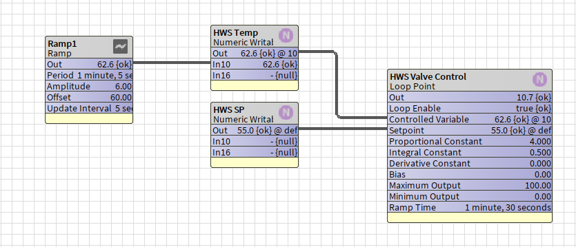
Real-World Example 2: Boiler Demand Control

The System:

Multiple heating zones with varying loads. A modulating boiler responds to 0-10V demand signal. You need to maintain flow temperature at 70°C despite constantly changing heat demand.

The Challenge:

• Morning startup: All zones call for heat simultaneously this causes a massive demand spike

• Mid-day: Some zones satisfied the demand drops quickly

• Boiler takes time to respond (thermal lag)

PI Control Solution:

• P term: Responds immediately to temperature drop from target (70°C to 65°C = big correction)

• I term: Accounts for sustained demand and eliminates temperature offset

• Result: Smooth modulation between 30-90% firing rate, maintaining 70°C ±1°C

Practical Tuning Guide (The Easy Way)

Most engineers overthink PID tuning. Here's a simple approach that works for 90% of HVAC applications.

Step 1: Choose Your Control Type

Start with PI control for almost everything. Set D = 0 initially.

Decision tree:

• Need exact setpoint with no offset? then Use PI

• System overshoots badly even with PI? then Try adding D (start very small)

• Simple system where ±1-2 degrees is fine? then P-only might work

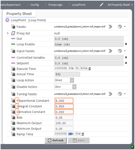
Step 2: Calculate Your Starting P-Gain (Kp)

Formula: Kp = (Output Range) / (Throttling Range)

Hot Water Example:

• Your valve control: 0-100% (Output Range = 100)

• When valve goes 0% to 100%, temperature changes by 20°C (Throttling Range = 20)

• Kp = 100 / 20 = 5

What this means: For every 1°C of error, the output changes by 5%

Real Example Calculation:

• Setpoint = 60°C, Current temp = 55°C the Error = 5°C

• Output = Kp × Error = 5 × 5 = 25% valve opening

Step 3: Set Your I-Gain (Ki) - For PI Control

Start conservative: Ki = 0.5 repeats/minute

What "repeats per minute" means:

If error stays constant for 1 minute, the I term will add the same amount that the P term initially added.

Example:

• Error = 5°C, P-gain = 5 the P term contributes 25% output immediately

• With Ki = 0.5, after 1 minute of constant 5°C error, I term adds another 12.5% (0.5 × 25%)

• After 2 minutes: I term adds 25% total (matching the P contribution)

Step 4: Test and Tune

Create a setpoint change and watch what happens:

Change setpoint from 60°C to 65°C and observe the response.

Step 5: Set Your Output Limits

Always define minimum and maximum output values:

• Minimum Output: Often 0%, but sometimes you need a minimum (e.g., 10% to keep valve from sticking)

• Maximum Output: Usually 100%, but might limit to 90% to prevent valve wear

Why this matters: These limits prevent integral windup (where the I term accumulates to crazy values when the output is maxed out).

Common Mistakes and How to Avoid Them

Mistake 1: Starting with PID Instead of PI

The problem: D term amplifies noise in sensor readings. Your temperature sensor might fluctuate ±0.2°C due to noise, and D term will react to these meaningless changes, causing erratic control.

The fix: Start with PI. Only add D if you have a real overshoot problem that PI can't solve. When you do add D, start very small (3-5 seconds).

Mistake 2: Setting Gains Too Aggressively

The problem: "I want fast response!" so You crank up Kp and Ki the System oscillates wildly then Occupants complain the Equipment wears out faster.

The fix: HVAC systems aren't race cars. Slower, stable control is better than fast, oscillating control. A loop that takes 15 minutes to settle smoothly is better than one that reaches setpoint in 5 minutes but bounces around for 30 minutes.

Mistake 3: Wrong Action Direction (Direct vs Reverse)

The problem: You set up your loop and the temperature runs away in the wrong direction!

Understanding Direct vs Reverse:

• Direct Action: Output increases when PV increases (cooling applications: higher temp then open cooling valve more)

• Reverse Action: Output increases when PV decreases (heating applications: lower temp then open heating valve more)

The fix: Think about your physical system. For heating: cold = need more heat = higher output = REVERSE action.

Mistake 4: Not Setting Bias Correctly

The rule of thumb:

• P-only control: Set bias to 50% (mid-point) so you can correct equally in both directions

• PI control: Set bias to 0% because the I term creates an automatic bias

Mistake 5: Ignoring System Physical Limits

The problem: You calculate Kp = 8, but your system physically can't respond that fast.

Reality check:

• Electric actuators take 60-120 seconds to fully stroke unless you have purchased fast acting

• Thermal systems have lag (heating a tank doesn't happen instantly)

• Temperature sensors take time to respond (thermal mass of the sensor itself)

The fix: Calculated gains are starting points. Watch the actual system behaviour and tune accordingly.

Quick Reference: Typical HVAC Starting Values

Remember: These are starting points! Every system is different. Watch the actual response and adjust accordingly. Remember watch and observe, time monitoring the control will be your friend.

Visual Troubleshooting Guide

When you plot your PV (process variable) vs. time, here's what different problems look like:

Good Control (Well Tuned PI):

• Smooth rise to setpoint

• Small or no overshoot (maybe 1-2% maximum)

• Settles at setpoint and stays there

• Minimal oscillation

Kp Too Low:

• Very slow, lazy rise toward setpoint

• Takes forever to get there

• No oscillation (too sluggish to oscillate)

• Fix: Increase Kp by 25-50%

Kp Too High:

• Rapid rise that overshoots setpoint

• Continuous oscillation above and below setpoint

• Oscillations don't die out

• Fix: Decrease Kp by 25-50%

Ki Too High:

• Good initial response

• Large overshoot past setpoint

• Swings back below setpoint

• May oscillate with decreasing amplitude

• Fix: Decrease Ki by 50%

Ki Too Low (or P-only):

• Rises nicely toward setpoint

• Gets close but stabilizes below setpoint (offset error)

• Never quite reaches target

• Fix: Increase Ki (double it)

Real-World Tuning Process (Step by Step)

Let's walk through tuning a hot water mixing valve controlling a buffer tank:

System Info:

• 500L buffer tank

• 3-port mixing valve (0-10V, 90-second stroke time)

• Target: 70°C

• Full valve range (0-100%) changes tank temp by approximately 25°C

Step 1: Calculate Initial Gains

Kp = Output range / Throttling range = 100 / 25 = 4

Ki = 0.5 repeats/minute (starting conservative)

Kd = 0 (starting with PI only)

Bias = 0 (using PI)

Step 2: First Test (Cold Start)

• Tank at 45°C, setpoint 70°C

• Error = 25°C, Output = Kp × Error = 4 × 25 = 100% (valve fully open - good!)

• Watch the response over 30 minutes

Step 3: Observe and Adjust

What we see: Temperature rises smoothly to 68°C then slows down dramatically. After 45 minutes, it's stuck at 69.2°C.

Diagnosis: Classic offset error - Ki is working but too slow

Action: Increase Ki from 0.5 to 1.0

Step 4: Second Test

What we see: Much better! Reaches 70°C in about 35 minutes, but overshoots to 71.5°C, then settles back to 70°C after minor oscillation.

Diagnosis: Ki slightly too aggressive for this thermal mass

Action: Reduce Ki from 1.0 to 0.7

Step 5: Final Test

What we see: Perfect! Smooth rise to 70°C in 38 minutes, tiny 0.3°C overshoot, settles at 70.0°C ± 0.1°C.

Final Settings: Kp = 4, Ki = 0.7, Kd = 0

Key Lesson: You made small adjustments based on actual behaviour. The loop is now perfectly tuned for this specific system. That's how it's done in the real world!

Summary: The 5 Things to Remember

1. Start with PI control for 90% of HVAC applications - Set Kd = 0. Only add D if PI alone can't prevent overshoot.

2. Calculate Kp = Output Range / Throttling Range - This is your starting point, not your final answer.

3. Start Ki conservatively at 0.5 repeats/minute - Increase if you have offset error. Decrease if you overshoot.

4. Watch the actual system response and tune iteratively - Make one change at a time. Test. Adjust. Repeat.

5. Stable control beats fast control every time - A loop that takes 20 minutes to settle smoothly is better than one that reaches setpoint in 3 minutes but oscillates for an hour.

Final Thoughts

PID control isn't rocket science - it's just three simple corrections working together. Don't overthink it. Start with the formulas above, watch what happens, and adjust based on what you see. After tuning a few loops, you'll develop intuition for it and be able to accurately guess the initial almost correct settings based on experience.

The best way to learn PID is to get hands-on. Set up a test loop with an oscillator ramp in workbench to throw a random controlled variable signal, try different settings, and watch the results.
You'll quickly see patterns emerge.

When in doubt: Start with PI, be conservative with your gains, and tune based on real-world performance. You've got this!